PCA

Chapters

• General Terms and tools
• PCA
  • PCA
  • Hebbian Learning
  • Kernel-PCA
• Source Separation
  • ICA
  • Infomax ICA
  • Second Order Source Separation
  • FastICA
• Stochastic Optimization
• Clustering
  • k-means Clustering
  • Pairwise Clustering
  • Self-Organising Maps
  • Locally Linear Embedding
• Estimation Theory
  • Density Estimation
    • Kernel Density Estimation
    • Parametric Density Estimation
  • Mixture Models - Estimation Models

PCA can be used as a compression algorithm(more correctly dimensionality reduction). Its goal is to extract vectors(components) out of the sample data which minimizes the squared distance of all points to that vector (aka variance). More specifically they are usually sorted by their variance. This could also be paraphrased as: “How well does this single vector explain all the data points” PCA can also be interpreted as¹:

• Maximize the variance of projection along each component.
• Minimize the reconstruction error (ie. the squared distance between the original data and its “estimate”).

All principal components are orthogonal to eachother. If you have \(n\) dimensions in your data, e.g. each data point is \(\mathbb{R}^{n}\), you will have \(n\) principal components.

It is possible to use any number of components to represent the original data. If your goal is the compression of data you will want to use a number of components \(< n\) in order to achieve a smaller data size. A common visualization of the usefulness of Principal Components is the Screeplot.

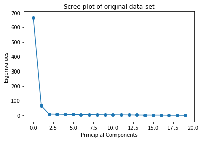
As can be seen the usefulness of the components drops of sharply in this example. Thereby with only very few components the original data can be approximated closely.

Generally PCA is based on the Eigenvalue problem

Projecting data

Each of the interesting components can be used to project the data into another vector space and later back.

Representation of $\underline{x}$ in the basis of PCs:

Reconstruction using projection onto first $M$ PCs:

projected_data = np.dot(centered_data,pcs[number_of_selected_pcs_using_screeplot:])

PCA as novelty filter

While the first principal components allow a close representation of the original data, the last principal components (those by which the data can be explained least) are useful for finding outliers (thus novelty filter).

A data point for which the least significant principal components are large is an outlier. (Data must have been previously centered for this to be true)

Principal Component Analysis (PCA)

As described above, the principal components minimize the variance

Hebbian Learning / Online PCA

Hebbian Learning is PCA but done on-the-fly (hence online). It can be used to find the most relevant PCs(Hebbian) or the least relevant PCs (Anti-Hebbian). It assumes centered data.

Variables: with learning rate \(\varepsilon\), \(\alpha \in \{1,...,p \}\), with number of data points \(p\), with \(\underline{x}^{(\alpha)} \in \mathbb{R}^N\)

Algorithm

• Initialize weights
• choose appropriate \(\varepsilon\)
• for \(\underline{x}^{(\alpha)} \in \underline{x}\)
  • \[\Delta\underline{w} = \varepsilon (\underline{w}^T\underline{x}^{(\alpha)})\underline{x}^{(\alpha)}\]
• end loop The weight vector \(w\) will converge to the Principal component with the largest eigenvalue. It is problematic that \(|w|\) will approach \(\infty\)

The intuition behind online PCA is that it works by averaging over all data

This is computationally expensive, because of the matrix multiplication \(\underline{w}^T\underline{x}\) . This is why in practice often a Taylor-Expansion is used.

Oyas Rule

Untuitive Euclidean normalization of the weights \(\underline{w}\)

which leads to

Sangers Rule

Sangers Rule allows having multiple weight vectors that approach the first \(M\) principal components. It essentially subtracts all weights of the previous principal components \(1..i\) making it converge to the next principal component.

Gram-Schmidt orthonormalization

Gram-Schmidt orthonormalization is about creating an orthonormalbasis, which in our case are the normalized PCs. After normalizing the first PC we look for a PC in the room orthogonal to the first. IN this case Oja’s rule is used for the orthonormalization.

Kernel PCA

Variables

• \(\underline a_k \in I\!R^p\) vector of eigenvalues for all dimensions. k is the instance of the datapoint.
• \(\underline e_k \in I\!R^N\) Eigenvector for each dimension.
• \(\underline K: p\times p\) matrix
• \(M\) number of dimensions in lowerdimensional space (feature space???) Kernel PCA transforms the data nonlinearly which then allows the usage of standard PCA. E.g. in an image each pixel may be a dimension which are mapped into lower dimensions. The lower dimensional feature space may be \(d{th}\) order monomials². is positive-semidefinite

Centering nonlinear transformation / feature vectors Uncentered feature vectors minus the mean. Nothing special here.

Centering kernel matrix

The kernel matrix must be centered by the row average column average and matrix average. Note the \(p^2\) entries in the matrix average (it’s a square matrix after all!).

Application

• Calculate kernel matrix \(\overset{\sim}{K}_{\alpha\beta} = k(\underline x^{(\alpha)},\underline x^{(\beta)}, \text{ with }\alpha,\beta\in \{1,...,p\}\)
• Center data (see above)

• Solve eigenvalue problem

  \[\frac{1}{p}\underline K \overset{\sim}{\underline \alpha}_k = \lambda_k\overset{\sim}{\underline \alpha}_k\]

• Normalize

  \[\underline a_k = \frac{1}{\sqrt{p\lambda_k}}\overset{\sim}{\underline \alpha}_k\]

• Calculate projections

  \[\sum^p_{\beta=1}a_k^{(\beta)}K_{\beta\alpha}\]

k corresponds to a scalar product in an M-dimensional space

Footnotes